Schwarz methods

Consider the following sample problem: \[\Delta u(x,y) = f(x,y), \quad (x,y) \in \Omega = [-1,1] \times [-1,1]\] \[u(x,y)=h(x,y), \quad (x,y) \in \partial \Omega\]

We'll discretize this into

\[A \vec{u} = \vec{f}, \quad A \in \mathbb{R}^{N \times N}\]

\[A \vec{u} = \vec{f}, \quad A \in \mathbb{R}^{N \times N}\]

If $N$ is very large, this can take a long time to find $\vec{u}$

Schwarz methods divide the domain into smaller problems

Schwarz methods divide the domain into smaller problems

\[\Delta u_1^n(x,y) = f(x,y), \quad (x,y) \in \Omega_1 = [-1,\alpha] \times [-1,1]\] \[u_1^n(\alpha,y)=u_2^{n-1}(\alpha,y)\] \[\Delta u_2^n(x,y) = f(x,y), \quad (x,y) \in \Omega_2 = [\beta,1] \times [-1,1]\] \[u_2^n(\beta,y)=u_1^{n-1}(\beta,y)\]

Schwarz methods divide the domain into smaller problems

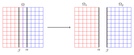
Schwarz methods divide the domain into smaller problems

Multiplicative Schwarz: solve one subdomain after the other

Additive Schwarz: solve both subdomains at the same time

Schwarz methods divide the domain into smaller problems

\[\begin{bmatrix} A_{11} & A_{1\Gamma} \\ A_{\Gamma 1} & A_{\Gamma \Gamma} & A_{\Gamma 2} \\ & A_{2 \Gamma} & A_{22} \end{bmatrix} \begin{bmatrix} \vec{u}_1 \\ \vec{u}_\Gamma \\ \vec{u}_2 \end{bmatrix} = \begin{bmatrix} \vec{f}_1 \\ \vec{f}_\Gamma \\ \vec{f}_2 \end{bmatrix}\]

Schwarz methods divide the domain into smaller problems

\[\begin{bmatrix} A_{11} & A_{1 \Gamma} \\ A_{\Gamma 1} & A_{\Gamma \Gamma} + T_{2 \to 1} \end{bmatrix} \begin{bmatrix} \vec{u}_1^{n+1} \\ \vec{u}_{1 \Gamma}^{n+1} \end{bmatrix} = \begin{bmatrix} \vec{f}_1 \\ \vec{f}_\Gamma \end{bmatrix} + \begin{bmatrix} ~ \\ -A_{\Gamma 2} \vec{u}_2^n + T_{2 \to 1} \vec{u}_{2 \Gamma}^n \end{bmatrix}\] \[\begin{bmatrix} A_{22} & A_{2 \Gamma} \\ A_{\Gamma 2} & A_{\Gamma \Gamma} + T_{1 \to 2} \end{bmatrix} \begin{bmatrix} \vec{u}_2^{n+1} \\ \vec{u}_{2 \Gamma}^{n+1} \end{bmatrix} = \begin{bmatrix} \vec{f}_2 \\ \vec{f}_\Gamma \end{bmatrix} + \begin{bmatrix} ~ \\ -A_{\Gamma 1} \vec{u}_1^n + T_{1 \to 2} \vec{u}_{1 \Gamma}^n \end{bmatrix}\]

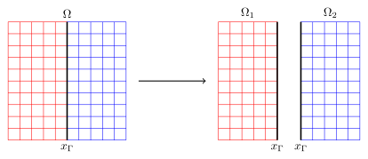
Optimized Schwarz methods

Boundary conditions transmit information between the two subdomains

We've used Dirichlet BCs

We could use Robin BCs instead

We could use Robin BCs instead

\[\Delta u_1^n(x,y) = f(x,y), \quad (x,y) \in \Omega_1 = [-1,0] \times [-1,1]\] \[\frac{\partial u_1^n}{\partial x} - p u_1^n(0,y)= \frac{\partial u_2^{n-1}}{\partial x} - p u_2^{n-1}(0,y)\] \[\Delta u_2^n(x,y) = f(x,y), \quad (x,y) \in \Omega_2 = [0,1] \times [-1,1]\] \[\frac{\partial u_2^n}{\partial x} - p u_2^n(0,y)= \frac{\partial u_1^{n-1}}{\partial x} - p u_1^{n-1}(0,y)\]

We could use Robin BCs instead

Now there's a choice in Robin parameter $p$, and this choice can be optimized

Optimization is done using Fourier analysis and finds the best $p$ for all Fourier modes

If you have a specific Fourier mode in mind, you can also pick the best $p$ for just that mode

Robin BCs aren't the only option for optimized BCs

Tangential BCs are also a popular choice, and give a second parameter $q$ to optimize \[\frac{\partial u_1^n}{\partial x} - p u_1^n(0,y) + q \frac{\partial u_1^n}{\partial y}=\] \[\frac{\partial u_2^{n-1}}{\partial x} - p u_2^{n-1}(0,y) + q \frac{\partial u_2^n}{\partial y}\]

But the best BCs are absorbing BCs, which are used in perfectly matched layers

These are dense, and correspond to Schur complements \[T_{2 \to 1} \to S_{2 \to 1} = -A_{\Gamma 2} A_{22}^{-1} A_{2 \Gamma},\] \[T_{1 \to 2} \to S_{1 \to 2} = -A_{\Gamma 1} A_{11}^{-1} A_{1 \Gamma}\]

These are dense, and correspond to Schur complements \[T_{2 \to 1} \to S_{2 \to 1} = -A_{\Gamma 2} A_{22}^{-1} A_{2 \Gamma},\] \[T_{1 \to 2} \to S_{1 \to 2} = -A_{\Gamma 1} A_{11}^{-1} A_{1 \Gamma}\]

This means they have about the same computation time as $M$ iterations, where $M$ is the size of the overlap

Adaptive transmission conditions

Finding optimized BCs requires Fourier analysis on each given problem

And the optimal BCs need Schur complements which are expensive to calculate

We want cheap, black box BCs

To get them, we'll find them adaptively

Let's look at the differences between iterates for a single sudomain

\[ \begin{bmatrix} A_{11} & A_{1 \Gamma} \\ A_{\Gamma 1} & A_{\Gamma \Gamma} + T_{2 \to 1} \end{bmatrix} \left ( \begin{bmatrix} \vec{u}_1^{n+1} \\ \vec{u}_{1 \Gamma}^{n+1} \end{bmatrix} - \begin{bmatrix} \vec{u}_1^n \\ \vec{u}_{1 \Gamma}^n \end{bmatrix} \right ) = \]\[ \begin{bmatrix} \vec{f}_1 \\ \vec{f}_\Gamma \end{bmatrix} + \begin{bmatrix} ~ \\ -A_{\Gamma 2} \vec{u}_2^n + T_{2 \to 1} \vec{u}_{2 \Gamma}^n \end{bmatrix} - \left (\begin{bmatrix} \vec{f}_1 \\ \vec{f}_\Gamma \end{bmatrix} + \begin{bmatrix} ~ \\ -A_{\Gamma 2} \vec{u}_2^{n-1} + T_{2 \to 1} \vec{u}_{2 \Gamma}^{n-1} \end{bmatrix} \right ) \]

Let's look at the differences between iterates for a single sudomain

\[ \begin{bmatrix} A_{11} & A_{1 \Gamma} \\ A_{\Gamma 1} & A_{\Gamma \Gamma} + T_{2 \to 1} \end{bmatrix} \begin{bmatrix} \vec{d}_1^{n+1} \\ \vec{d}_{1 \Gamma}^{n+1} \end{bmatrix} = \]\[ \begin{bmatrix} ~ \\ -A_{\Gamma 2} \vec{d}_2^n + T_{2 \to 1} \vec{d}_{2 \Gamma}^n \end{bmatrix} \]

We then perform what's known as static condensation by noting that \[A_{11} \vec{d}_1^{n+1} = -A_{\Gamma 1} \vec{d}_{1 \Gamma}^{n+1} \]

This leads to

\[(A_{\Gamma \Gamma} + S_{1 \to 2} + T_{2 \to 1}) \vec{d}_{1 \Gamma}^{n+1} = (T_{2 \to 1} - S_{2 \to 1}) \vec{d}_{2 \Gamma}^n \]

\[ \vec{y}^{n+1} = E_2 \vec{d}_{2 \Gamma}^n = -A_{\Gamma 2} \vec{d}_2^n + T_{2 \to 1} \vec{d}_{2 \Gamma}^n \]

\[ \vec{y}^{n+1} = E_2 \vec{d}_{2 \Gamma}^n = -A_{\Gamma 2} \vec{d}_2^n + T_{2 \to 1} \vec{d}_{2 \Gamma}^n \]

At every other iteration, we're going to update $E_2$

\[ E_2 \to E_2 - \frac{ \vec{y} \vec{d}^\top }{ \Vert \vec{d} \Vert^2 } \]

\[ E_2 \to E_2 - \frac{ \vec{y} \vec{d}^\top }{ \Vert \vec{d} \Vert^2 } \]

With each iteration, there's a new pair of $\vec{y}$ and $\vec{d}$

We can apply a modified Gram-Schmidt process to the vectors $\vec{d}$, making the vectors $\vec{w}$

Through this process, the vectors $\vec{y}$ get modified as well, to the vectors $\vec{v}$

\[ E_2 \to E_2 - V W^\top \]

Since $V = E_2 W$, this is equivalent to \[ E_2 \to E_2 \left ( I - W W^\top \right ) \]

We generate a low rank approximation of $E_2$

To make the optimized BCs, we subtract this from $T_{2 \to 1}$

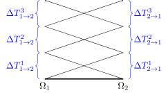
The transmission conditions $T_{2 \to 1}$ and $T_{1 \to 2}$ now change iteratively

Recall: \[(A_{\Gamma \Gamma} + S_{1 \to 2} + T_{2 \to 1}) \vec{d}_{1 \Gamma}^{n+1} = (T_{2 \to 1} - S_{2 \to 1}) \vec{d}_{2 \Gamma}^n \]

The vectors $\vec{d}$ lie in a Krylov subspace

They satisfy an implicit Galerkin condition

There's also the option to update the BCs at every iteration

Adaptive Optimized Schwarz Methods (AOSMs)

1. Initial guesses

Make initial choices of $\vec{u}_{1 \Gamma}^0$, $T_{1 \to 2}^1$ and $T_{2 \to 1}^1$

Find $\vec{u}_1^0 = A_{11}^{-1} \left ( \vec{f}_1 - A_{1 \Gamma} \vec{u}_{1 \Gamma}^0 \right )$

Solve \[ \begin{bmatrix} A_{22} & A_{2 \Gamma} \\ A_{\Gamma 2} & A_{\Gamma \Gamma} + T_{1 \to 2}^1 \end{bmatrix} \begin{bmatrix} \vec{u}_{2}^1 \\ \vec{u}_{2 \Gamma}^1 \end{bmatrix} = \begin{bmatrix} \vec{f}_2 \\ \vec{f}_\Gamma \end{bmatrix} + \begin{bmatrix} ~ \\ -A_{\Gamma 1} \vec{u}_1^0 + T_{1 \to 2}^1 \vec{u}_{1 \Gamma}^0 \end{bmatrix} \]

2. Seed Krylov subspace

Solve \[ \begin{bmatrix} A_{11} & A_{1 \Gamma} \\ A_{\Gamma 1} & A_{\Gamma \Gamma} + T_{2 \to 1}^1 \end{bmatrix} \begin{bmatrix} \vec{u}_{1}^2 \\ \vec{u}_{1 \Gamma}^2 \end{bmatrix} = \begin{bmatrix} \vec{f}_1 \\ \vec{f}_\Gamma \end{bmatrix} + \begin{bmatrix} ~ \\ -A_{\Gamma 2} \vec{u}_2^1 + T_{2 \to 1}^1 \vec{u}_{2 \Gamma}^1 \end{bmatrix} \]

Calculate $\vec{d}_{1 \Gamma}^2 = \vec{u}_{1 \Gamma}^2 - \vec{u}_{1 \Gamma}^0$ and $\vec{d}_{1}^2 = \vec{u}_{1}^2 - \vec{u}_{1}^0$

2. Seed Krylov subspace

Calculate $\vec{d}_{1 \Gamma}^2 = \vec{u}_{1 \Gamma}^2 - \vec{u}_{1 \Gamma}^0$ and $\vec{d}_{1}^2 = \vec{u}_{1}^2 - \vec{u}_{1}^0$

Normalize $\vec{d}_{1 \Gamma}^2$ using $\alpha_1^2$ such that $\vec{w}_1^2 = \alpha_1^2 \vec{d}_{1 \Gamma}^2$ and calculate \[ \vec{v}_1^2 = \alpha_1^2 \left ( -A_{\Gamma 1} \vec{d}_1^2 + T_{1 \to 2}^1 \vec{d}_{1 \Gamma}^2 \right ) \]

Update $T_{1 \to 2}^1$: \[ T_{1 \to 2}^2 = T_{1 \to 2}^1 + \Delta T_{1 \to 2}^2 = T_{1 \to 2}^1 - \vec{v}_1^2 \left ( \vec{w}_1^2 \right )^\top \]

2. Seed Krylov subspace

Solve

\[ \begin{bmatrix} A_{22} & A_{2 \Gamma} \\ A_{\Gamma 2} & A_{\Gamma \Gamma} + T_{1 \to 2}^2 \end{bmatrix} \begin{bmatrix} \vec{d}_{2}^3 \\ \vec{d}_{2 \Gamma}^3 \end{bmatrix} \]

\[ = \begin{bmatrix} ~ \\ -A_{\Gamma 1} \vec{d}_1^2 + T_{1 \to 2}^2 \vec{d}_{1 \Gamma}^2 - \Delta T_{1 \to 2}^2 \left ( \vec{u}_{2 \Gamma}^1 - \vec{u}_{1 \Gamma}^0 \right ) \end{bmatrix} \]

2. Seed Krylov subspace

Solve

\[ \begin{bmatrix} A_{22} & A_{2 \Gamma} \\ A_{\Gamma 2} & A_{\Gamma \Gamma} + T_{1 \to 2}^2 \end{bmatrix} \begin{bmatrix} \vec{d}_{2}^3 \\ \vec{d}_{2 \Gamma}^3 \end{bmatrix} \]

\[ = \langle \vec{w}_1^2, \vec{u}_{2 \Gamma}^1 - \vec{u}_{1 \Gamma}^0 \rangle \begin{bmatrix} ~ \\ \vec{v}_1^2 \end{bmatrix} \]

2. Seed Krylov subspace

Normalize $\vec{d}_{2 \Gamma}^3$ using $\alpha_2^3$ such that $\vec{w}_2^3 = \alpha_2^3 \vec{d}_{2 \Gamma}^3$ and calculate \[ \vec{v}_2^3 = \alpha_2^3 \left ( -A_{\Gamma 2} \vec{d}_2^3 + T_{2 \to 1}^1 \vec{d}_{2 \Gamma}^3 \right ) \]

Update $T_{2 \to 1}^1$: \[ T_{2 \to 1}^3 = T_{2 \to 1}^1 - \vec{v}_2^3 \left ( \vec{w}_2^3 \right )^\top \]

3. Iterate

Solve for $\vec{d}_i^n$ and $\vec{d}_{i \Gamma}^n$

Apply modified Gram-Schmidt to find $\vec{v}_i^n$ and $\vec{w}_i^n$

Update $T_{i \to j}^n$ using $\vec{v}_i^n \left ( \vec{w}_i^n \right )^\top$

Woodbury matrix identity

The updates to $T_{1 \to 2}^n$ and $T_{2 \to 1}^n$ are low rank

In order to preserve any matrix factorizations, we can use the Woodbury matrix identity to apply these low rank updates

\[(A - V W^\top) \vec{u} = \vec{f},\] \[\vec{u} = A^{-1} \vec{f} + A^{-1} V (I_{k \times k} - W^\top A^{-1} V)^{-1} W^\top A^{-1} \vec{f}\]

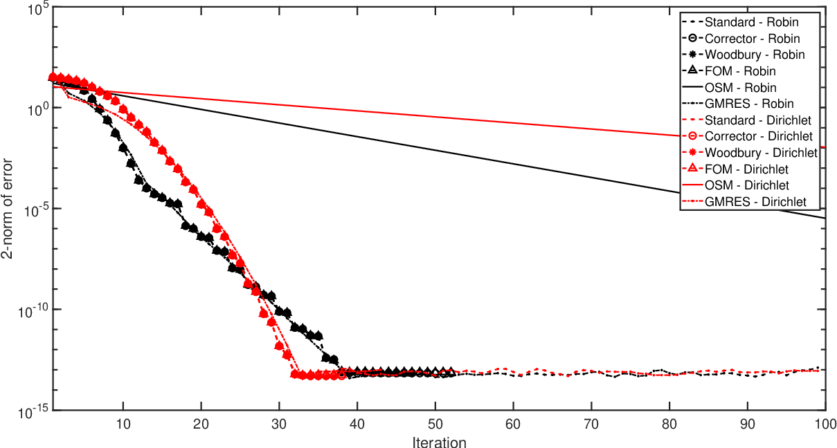
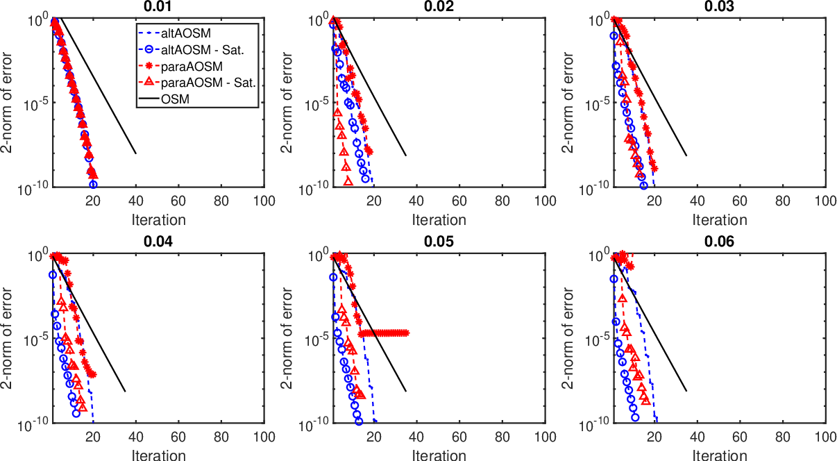
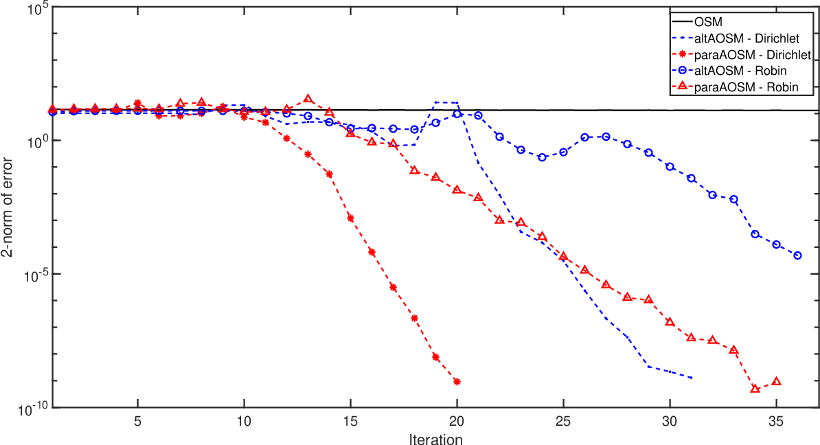
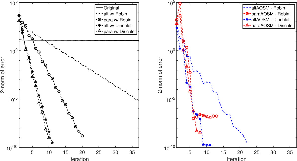
Numerical experiments

Recall the sample problem: \[\Delta u(x,y) = f(x,y), \quad (x,y) \in \Omega = [-1,1] \times [-1,1]\] \[u(x,y)=h(x,y), \quad (x,y) \in \partial \Omega\]

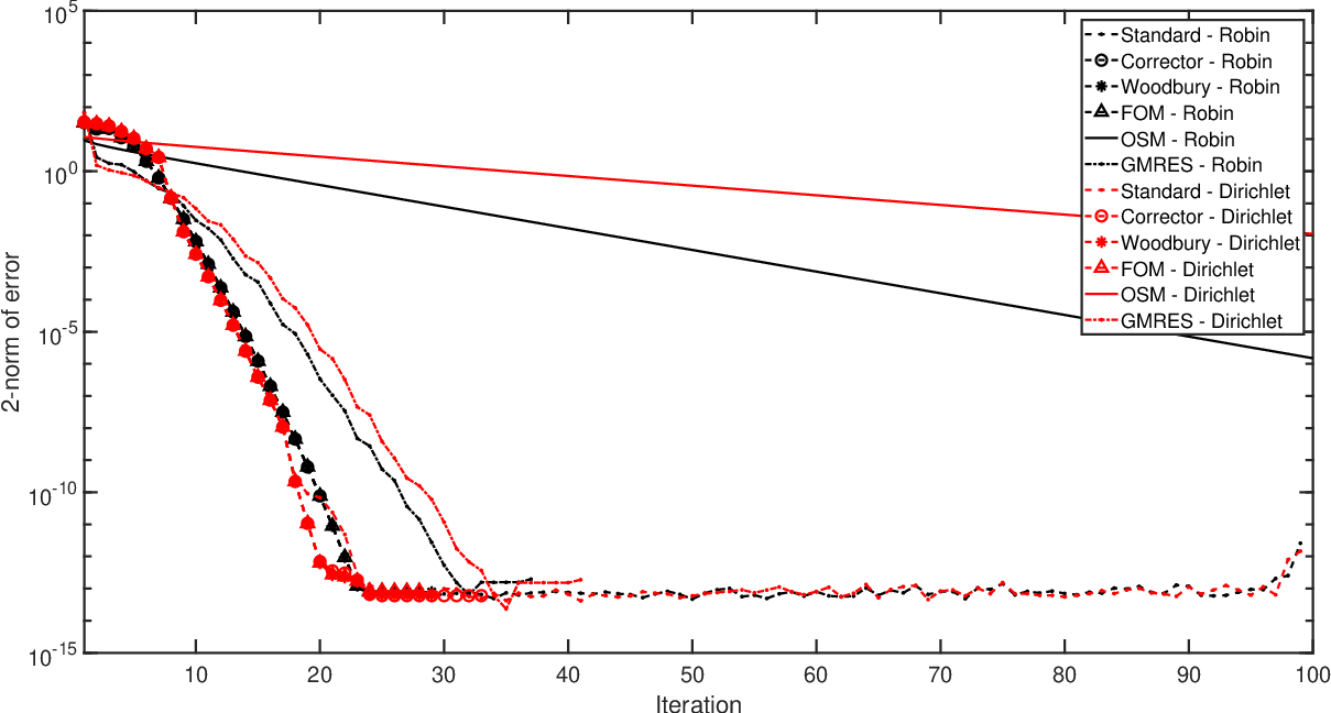
Let's apply AOSMs to this problem

\[ u_t(x,y,t) = \Delta u(x,y,t), \quad (x,y) \in \Omega = [-1,1] \times [-1,1], \ t \in [0,T] \] \[ u(x,y,0) = u_0(x,y), \quad (x,y) \in \Omega, \] \[ u(x,y,t) = h(x,y), \quad (x,y) \in \partial \Omega, \ t \in [0,T] \]

\[\frac{u_{n+1} - u_n}{\Delta t} = A u_{n+1}\] \[(I - \Delta t A) u_{n+1} = u_n\]

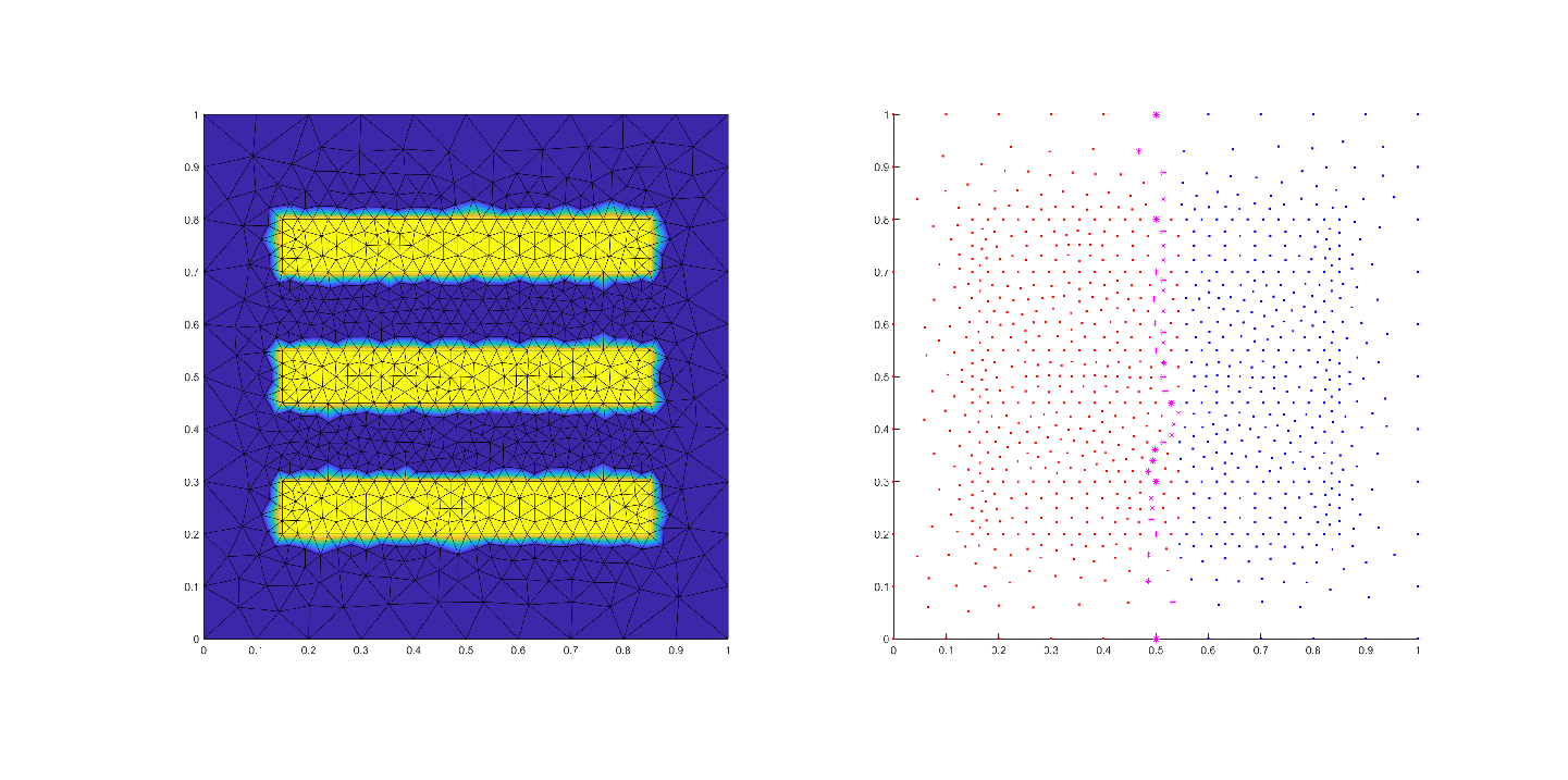
\[ \nabla (\alpha(x,y) \cdot \nabla u(x,y) ) = f(x,y), \quad (x,y) \in \Omega = [-1,1] \times [-1,1], \] \[ u(x,y) = h(x,y), \quad (x,y) \in \partial \Omega, \]

Solve this using FEM software